Types and Operations
A matrix is an array of numbers (elements) presented in a standard form such as the one below. If you wish to use one in an algebraic expression, it is conventional to use a capital letter as an identifier.

The order of a matrix is the number of rows multiplied by the number of columns e.g the order of the above matrix is [2x3] (pronounced two by three)
Intuitively, a matrix is called square if it has the same number of rows as columns, and we can also say column matrix to mean a matrix with only one column, and row matrix for a matrix with only one row.
Operations
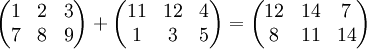
- Adding Matrices
Adding matrices is as you would expect: take a number from the first matrix and add it to the number in the corresponding position in the second matrix and place the result in the third matrix in the same position. This has the obvious limitation that only matrices of the same order can be added together.
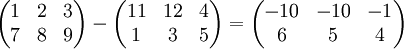
- Subtracting Matrices
Subtracting matrices is also as you would expect and is the exact opposite of adding matrices (see above).
- Multiplying Matrices
Unfortunately, multiplying matrices is not as expected. The most simple way of defining multiplication of matrices is to give an example in algebraic form.
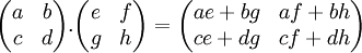
As above, to find the value of each element in the resulting matrix, you have to take the sum of the row in the first matrix multiplied by the column in the second matrix. Because of this, matrices can only be multiplied together if they are conformable - i.e. if the second matrix has the same number of rows as there are columns in the first matrix. A quick rule of thumb is that if you have an [axb] order matrix you can multiply it by a [bxc] matrix to obtain an [axc] matrix.

The other major problem with multiplying matrices is that it is not, in general, commutative. This means that  . This is very counterintuitive as multiplication between real numbers is not like this. As an example, if we multiply the above two matrices the other way around, we get a different matrix.

Of course there exist matricies that do 'commute'. For example take the product of the identity matrix  with any other square matrix, of the same dimension, and these clearly commute.
Multiplication by a scalar is easier; you simply multiply the number by every element in the matrix. For example:

- Dividing Matrices
Division of matrices is not defined. However we can multiply by the inverse matrix to achieve the same result. See below for how to find the inverse of a matrix.
Identity Matrices
The identity matrix is the matrix which when multiplied by another matrix returns that matrix - in other words it is the equivalent of the real number 1. Because this can only happen with square matrices, an identity matrix is a square matrix which apart from a diagonal line of ones from top left to bottom right consists only of zeros. The three by three identity matrix known as  is thus:

Zero Matrices
The zero matrix or null matrix is denoted  , and it's simply a matrix populated exclusively by zeros.
Both of the following matrices are called .


Naturally, for any matrix M,
 and
and 
Inverse Matrices
If you have two matrices such that  then you can think to yourself that A is equal to
  , which is analogous to
  . However, since we do not specifically define division for matrices, we must always use the notation B-1 instead of 1/B. So we have:
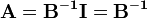
A matrix X-1 is called the inverse matrix of X - if you multiply the two together you get the identity matrix.
2x2 Matrices
- Inverse
For two by two matrices the process of finding an inverse is very simple:

This implies that not all square matrices do have an inverse, since if ad − bc is zero then the inverse will be undefined. A matrix with no inverse is known as singular.
The formula above is derived as follows:

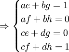


Taking out a factor of  gives:

- Determinant
This part of the equation (ad − bc) is know as the determinant of the matrix and has many other uses which will be gone into later. It is written in several different ways including:

- Transpose
For the matrix  , its transpose is denoted MT and is equal to
This is the end of first primer. In the next primer, we will discuss 3x3 matrices and solving system of equations and matrices transformations.
References
The content of this article is taken from the opensource and public wiki books at:
http://en.wikibooks.org/wiki/A-level_Mathematics/FP1/Matrices
Comments
Post a Comment